SPRING Help Page
With an increasing number of genomic data (DNA, RNA, and protein
sequences) being available, the study of genome rearrangement has
received a lot of attention in computational biology and bioinformatics
because of its applications in the measurement of evolutionary difference
between two species.
In this study, the considered chromosomes are usually denoted
by permutations of ordered and signed integers with each integer
representing an identical gene in the chromosomes and
its sign (e.g., + or -) indicating the transcriptional orientation.
Here, we use permutation and chromosome interchangeably.
Given two permutations representing two linear/circular chromosomes,
the genome rearrangement study is to compute the
rearrangement distance that is defined to be a
minimum number of rearrangement operations required to
transform one chromosome into another.
The commonly used rearrangement operations affecting
a permutation include reversals
(also called inversions),
transpositions,
block-interchanges (i.e., generalized
transpositions) and even their
combinations.
Reversals act on the permutation by inverting a block of consecutive
integers into the reverse order and also changing the
sign of each integer,
and transpositions act by swapping
two contiguous (or adjacent) blocks of consecutive integers.
Conceptually, block-interchanges are a generalization of
transpositions with allowing the swapped blocks
to be not necessarily adjacent in the permutation.
Currently, many existing tools
have focused on inferring an optimal series of
reversals
or an optimal series of block-interchanges for
transforming one chromosome into another.
Here, we have developed a web server, called
SPRING (short for Sorting Permutation by
Reversals and block-INterchanGes),
to compute the rearrangement distance as well as an optimal scenario
between two permutations of representing linear/circular chromosomes
using reversals and/or block-interchanges.
If both reversals and block-interchanges are considered
together, SPRING adopts a strategy of unequal weight
by using weight 1 for reversals and weight 2 for block-interchanges.
This is mainly due to the following reasons.
First, reversals have been favored as more frequent
rearrangement operations when compared with block-interchanges.
Second, a reversal affecting the chromosome removes at most
two breakpoints, whereas a block-interchange removes at
most four, where a breakpoint denotes two adjacent genes
(g1, g2) in a chromosome that does not appear consecutively
as either (g1, g2) or (-g2, -g1)
in another chromosome.
Third, the rearrangement distance involving both reversals and block-interchanges
can currently be computed in polynomial time only when the weight of reversals is
1 and the weight of block-interchanges is 2.
For this combination of reversals and block-interchanges,
we have designed an efficient algorithm
to compute the rearrangement distance between
two permutations and also generate a minimum weighted series of
reversals and block-interchanges required to transform one
permutation into another.
In addition, SPRING computes the breakpoint
distance between two permutations, which can be used to compare
with the rearrangement distance to see whether they are correlated or not,
where the breakpoint distance is
the number of breakpoints between the two permutations.
By integrating two existing programs,
respectively called
Mauve and
PHYLIP,
SPRING can accept not only gene-order data but also
sequence data as its input, and can output the evolutionary
trees that are inferred based on the calculated breakpoint and
rearrangement distances.
In particular, if the input is sequence data,
SPRING will automatically search for
the identical landmarks that are the homologous/conserved regions
shared by all the input sequences.
Here, we adopt the so-called LCBs (Locally Collinear Blocks) for representing
the landmarks in chromosomes.
The LCB is defined as a collinear (consistent) set of the multi-MUMs
where the multi-MUMs are the exactly matching subsequences
shared by all the considered chromosomes that occur only once in
each chromosome and that are bounded on either side by mismatched
nucleotides.
Then its weight is the sum of the lengths of the contained
multi-MUMs.
The weight of an LCB can serve as a measure of confidence that
it is a true homologous region rather than a random match.
By selecting a higher minimum weight, SPRING can identify the larger LCBs
that are truly involved in genome rearrangement, whereas by selecting a
lower minimum weight, SPRING can trade some specificity for sensitivity
to identify the smaller LCBs that are possibly involved in
genome rearrangement.
For the details about LCB, we refer users to the paper
by Darling et al. (2004).
The rest sections of this page are:
- Usage of SPRING
- Experimental Results
- CPU Time Usage
- FASTA and FASTA-like Format Descriptions
- Some Collection of Testing Examples
- Contact information
- References
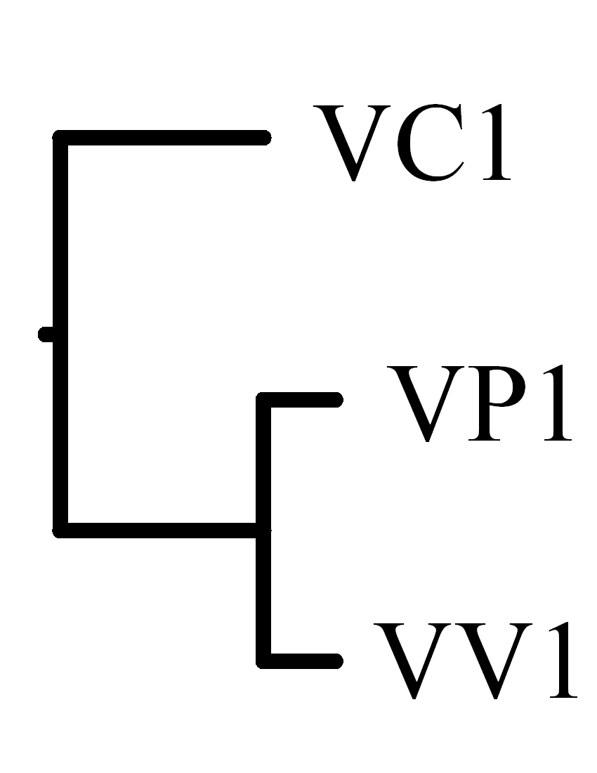
SPRING accepts genomic sequences or gene/landmark orders as its input.
If the input is genomic sequence data, then users can follow the
steps described below to execute SPRING.
-
Enter or paste a set of sequences in FASTA format
(1),
or simply upload a plain text file of sequences in FASTA format
(2).
-
Choose the rearrangement operations
(3), which can be either
reversals (inversions), block-interchanges or both.
-
Specify a minimum multi-MUM length (4)
whose default is set to log2n,
where n is the average length of input sequences.
-
Specify a minimum LCB (Locally Collinear Block) weight
(5) whose
default is set to 3*(minimum multi-MUM length).
-
Select the chromosome type (6) according to
the type of the input chromosomes that can be either linear or circular.
- Determine if the optimal rearrangement scenarios computed
by SPRING are also shown in the output page
(7).
-
Check email box and simultaneously enter an email address
(8), if users would like to
run SPRING in a batch way.
In this way, users will be notified of the output via email
when the submitted job is finished.
This email check is optional but recommended if the sequences
users enter/upload are large-scale.
- Click "Submit" button to run SPRING
(9).
If the input is gene-/landmark-order data,
then users follow the following steps to run SPRING.
-
Input or paste a set of gene/landmark orders in
FASTA-like format (10),
or simply upload a plain text file of gene/landmark orders in
FASTA-like format (11).
-
Choose the rearrangement operations
(12), which can be either reversals
(inversions), block-interchanges or both.
Note that the signs of the input gene/landmark orders will be
ignored by SPRING if the chosen rearrangement operations are
only block-interchanges.
-
Select the chromosome type (13) according to
the type of the input chromosomes that can be either linear or circular.
- Determine if the optimal rearrangement scenarios computed
by SPRING are also shown in the output page
(14).
- Click "Submit" button to run SPRING
(15).
Output
If the input is a set of chromosomal sequences, then SPRING will first
output the order of the identified common LCBs shared by all
the input sequences, and then output the rearrangement distance matrix
(in which each entry denotes the rearrangement distance between
a pair of two input chromosomes), as well as the breakpoint distance matrix.
The breakpoint distances can be used to compare with the rearrangement
distances to see whether they are correlated or not.
In addition, SPRING shows two phylogenetic trees that are reconstructed
based on the rearrangement and breakpoint distance matrixes, respectively,
using a program of neighbor-joining method from the
PHYLIP package.
In each of the identified LCB orders, users can see its detailed
information just by clicking the associated link, such as
the position (denoted by left and right end coordinates),
length and weight of each LCB, and the overall coverage of all LCBs.
It should be noted that if both the left and right coordinates of
an identified LCB are negative values, then this LCB is
the inverted region on the opposite strand of the given sequence
and the sign of its corresponding integer is "-".
If users choose to show the optimal scenarios before running SPRING,
then they can view the optimal scenario between any pair of two
input sequences just by clicking the link associated with each entry
in the computed distance matrix.
In the display of an optimal scenario, the operations of reversals
are marked with green color and those of block-interchanges with
red and blue colors.
Here is an example of the
output we obtained by running SPRING with the
second chromosomes of three Vibrio species,
including V. cholerae, V. parahaemolyticus and
V. vulnificus.
On the other hand, if the input is a set of gene/landmark orders,
SPRING just outputs the breakpoint and rearrangement distance matrixes
along with their evolutionary trees, and the optimal scenarios
between pairs of any two gene/landmark orders.
Here is an example of the
output we obtained by running SPRING with the gene orders of
two gamma-proteobacteria (i.e., Shewanella oneidensis and
Wigglesworthia glossinidia).
To validate SPRING, we have tested it with two sets of chromosomal
sequences and a set of gene orders for detecting the
evolutionary relationships of the input species.
All the tests were run using SPRING with default parameters and
their detailed input data and experimental results can be accessed
and referred in this help page.
Genome rearrangements by reversals have recently been studied in
gamma-proteobacterial complete genomes by comparing the
order of a reduced set of genes on the chromosome
(Belda et al., 2005).
For our purpose, we selected 11 gamma-proteobacterial complete
sequences (see Table 1 for their sequence information)
and tried to use SPRING to infer their phylogenetic tree
by considering reversals and block-interchanges together.
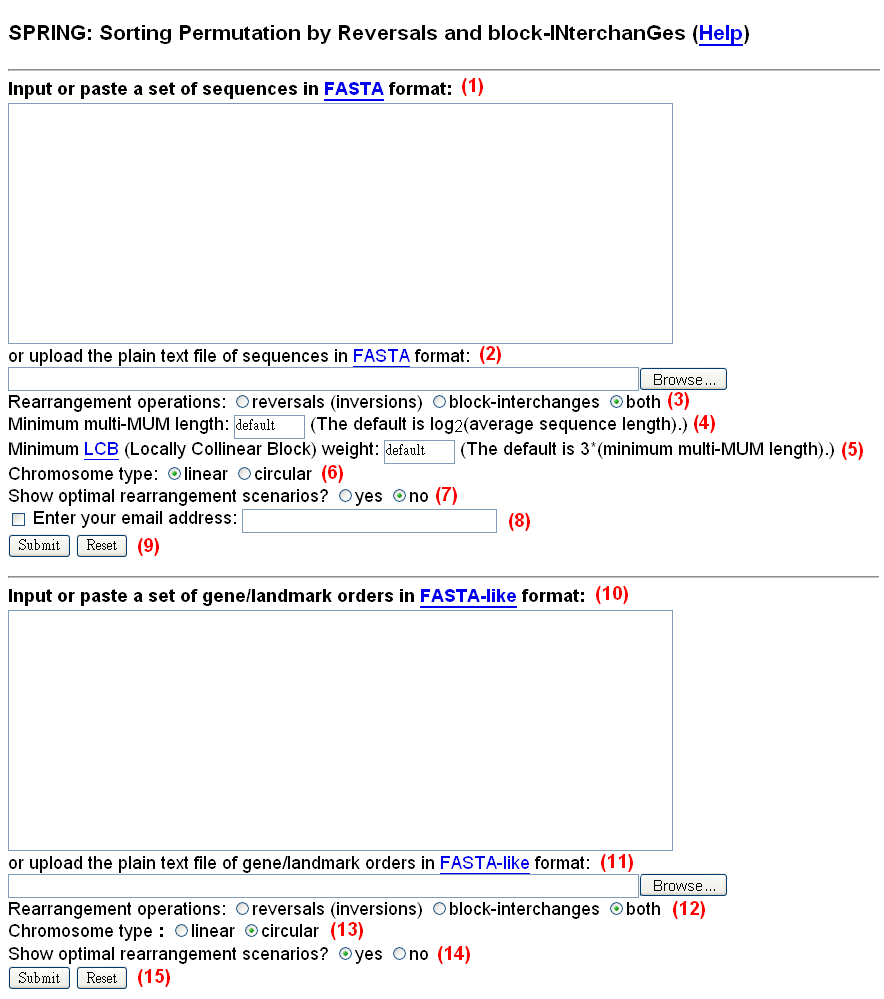
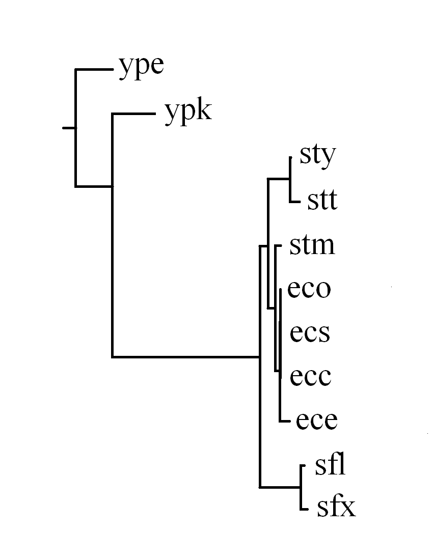
The experimental results, including the breakpoint/rearrangement
distance matrixes and their constructed phylogenetic trees, are
shown in Table 2.
Consequently, there are 58 identified LCBs in total and the topologies of
the constructed phylogenetic trees based on the breakpoint
and rearrangement distance matrixes respectively are very similar.
In fact, we calculated the correlation coefficient between
the breakpoint and rearrangement distance matrixes that
is 0.996, indicating high correlation between these two distances.
Table 1:
The sequence information of 11 gamma-proteobacteria
| Accession NO |
Species |
Abbreviation |
Size (Mbp) |
| NC_000913 |
Escherichia coli K12 |
eco |
4.6 |
| NC_002695 |
Escherichia coli O157:H7 |
ecs |
5.5 |
| NC_002655 |
Escherichia coli O157:H7 EDL933 |
ece |
5.5 |
| NC_004431 |
Escherichia coli CFT073 |
ecc |
4.6 |
| NC_004741 |
Shigella flexneri 2a str. 2457T |
sfx |
4.6 |
| NC_004337 |
Shigella flexneri 2a str. 301 |
sfl |
4.7 |
| NC_003197 |
Salmonella typhimurium LT2 |
stm |
4.8 |
| NC_003198 |
Salmonella enterica subsp. enterica serovar Typhi str. CT18 |
sty |
4.8 |
| NC_004631 |
Salmonella enterica subsp. enterica serovar Typhi Ty2 |
stt |
4.8 |
| NC_003143 |
Yersinia pestis CO92 |
ype |
4.6 |
| NC_004088 |
Yersinia pestis KIM |
ypk |
4.6 |
Table 2:
The breakpoint and rearrangement distance matrixes
of 11 gamma-proteobacteria
(click this link
for the detailed SPRING result).
| Breakpoint distance |
|
ece |
eco |
ecs |
ecc |
sfl |
sfx |
stm |
sty |
stt |
ype |
ypk |
| ece | - | 2 | 2 | 2 | 13 | 14 | 4 | 9 | 11 | 51 | 43 |
| eco | 2 | - | 0 | 0 | 12 | 13 | 2 | 7 | 9 | 49 | 42 |
| ecs | 2 | 0 | - | 0 | 12 | 13 | 2 | 7 | 9 | 49 | 42 |
| ecc | 2 | 0 | 0 | - | 12 | 13 | 2 | 7 | 9 | 49 | 42 |
| sfl | 13 | 12 | 12 | 12 | - | 2 | 14 | 18 | 19 | 53 | 47 |
| sfx | 14 | 13 | 13 | 13 | 2 | - | 15 | 18 | 19 | 53 | 47 |
| stm | 4 | 2 | 2 | 2 | 14 | 15 | - | 6 | 8 | 49 | 42 |
| sty | 9 | 7 | 7 | 7 | 18 | 18 | 6 | - | 2 | 47 | 43 |
| stt | 11 | 9 | 9 | 9 | 19 | 19 | 8 | 2 | - | 48 | 44 |
| ype | 51 | 49 | 49 | 49 | 53 | 53 | 49 | 47 | 48 | - | 23 |
| ypk | 43 | 42 | 42 | 42 | 47 | 47 | 42 | 43 | 44 | 23 | - |
|
|
| Rearrangement distance |
|
ece |
eco |
ecs |
ecc |
sfl |
sfx |
stm |
sty |
stt |
ype |
ypk |
| ece | - | 1 | 1 | 1 | 8 | 9 | 2 | 6 | 7 | 37 | 33 |
| eco | 1 | - | 0 | 0 | 7 | 8 | 1 | 5 | 6 | 36 | 32 |
| ecs | 1 | 0 | - | 0 | 7 | 8 | 1 | 5 | 6 | 36 | 32 |
| ecc | 1 | 0 | 0 | - | 7 | 8 | 1 | 5 | 6 | 36 | 32 |
| sfl | 8 | 7 | 7 | 7 | - | 1 | 8 | 12 | 13 | 43 | 39 |
| sfx | 9 | 8 | 8 | 8 | 1 | - | 9 | 11 | 12 | 42 | 40 |
| stm | 2 | 1 | 1 | 1 | 8 | 9 | - | 4 | 5 | 35 | 31 |
| sty | 6 | 5 | 5 | 5 | 12 | 11 | 4 | - | 1 | 35 | 33 |
| stt | 7 | 6 | 6 | 6 | 13 | 12 | 5 | 1 | - | 36 | 34 |
| ype | 37 | 36 | 36 | 36 | 43 | 42 | 35 | 35 | 36 | - | 15 |
| ypk | 33 | 32 | 32 | 32 | 39 | 40 | 31 | 33 | 34 | 15 | - |
|
|
(2)
Chromosomal Sequences of Three Human Vibrio Pathogens
V. vulnificus is an etiologic agent for severe
human infection acquired through wounds or contaminated seafood and
shares morphological and biochemical characteristics with other human
Vibrio pathogens,
including V. cholerae and V. parahaemolyticus.
Currently, the genomes of these three Vibrio species, each consisting of two
circular chromosomes (see Table 3 for their sequence information),
have be sequenced and it has been reported that
V. vulnificus is closer to V. parahaemolyticus
than to V. cholerae from the evolutionary viewpoint
(Chen et al., 2003; Lin et al., 2005;
Lu et al., 2005).
Table 3: The sequence information of three pathogenic
Vibrio species, each with two circular Chromosomes
| Accession NO |
Species |
Chromosome |
Size (Mbp) |
| NC_005139 |
V. vulnificus YJ016 |
1 (VV1) |
3.4 |
| NC_005140 |
V. vulnificus YJ016 |
2 (VV2) |
1.9 |
| NC_004603 |
V. parahaemolyticus RIMD 2210633 |
1 (VP1) |
3.3 |
| NC_004605 |
V. parahaemolyticus RIMD 2210633 |
2 (VP2) |
1.9 |
| NC_002505 |
V. cholerae El Tor N16961 |
1 (VC1) |
3.0 |
| NC_002506 |
V. cholerae El Tor N16961 |
2 (VC2) |
1.0 |
In this experiment, we re-inferred their evolutionary
relationships by applying SPRING to their complete sequences
in a way of chromosome by chromosome.
The adopted rearrangement operations include reversals and
block-interchanges.
Tables 4 and 5 show the breakpoint and block-interchange
distance matrixes we computed for the first and second chromosomes,
respectively.
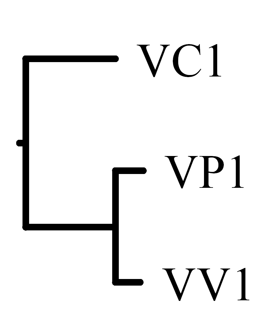
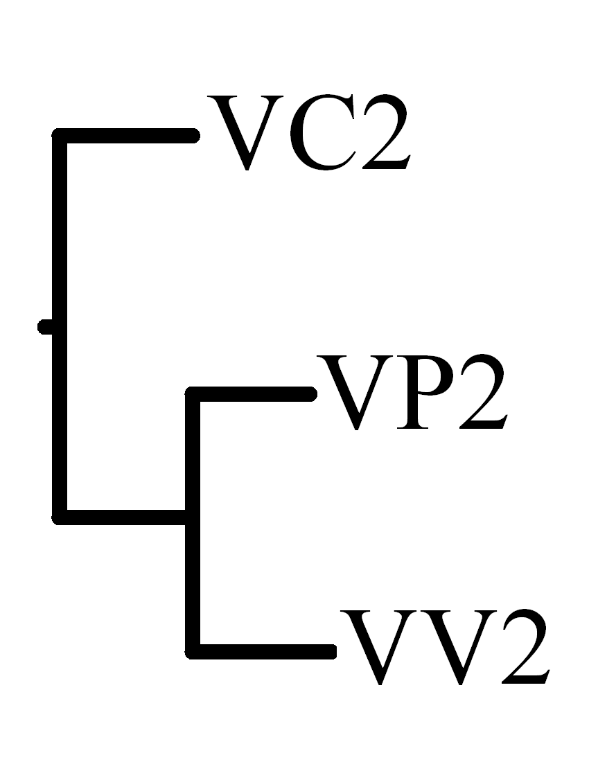
In the experimental results, we found that the optimal rearrangement
scenarios calculated by SPRING have no block-interchanges
but only reversals.
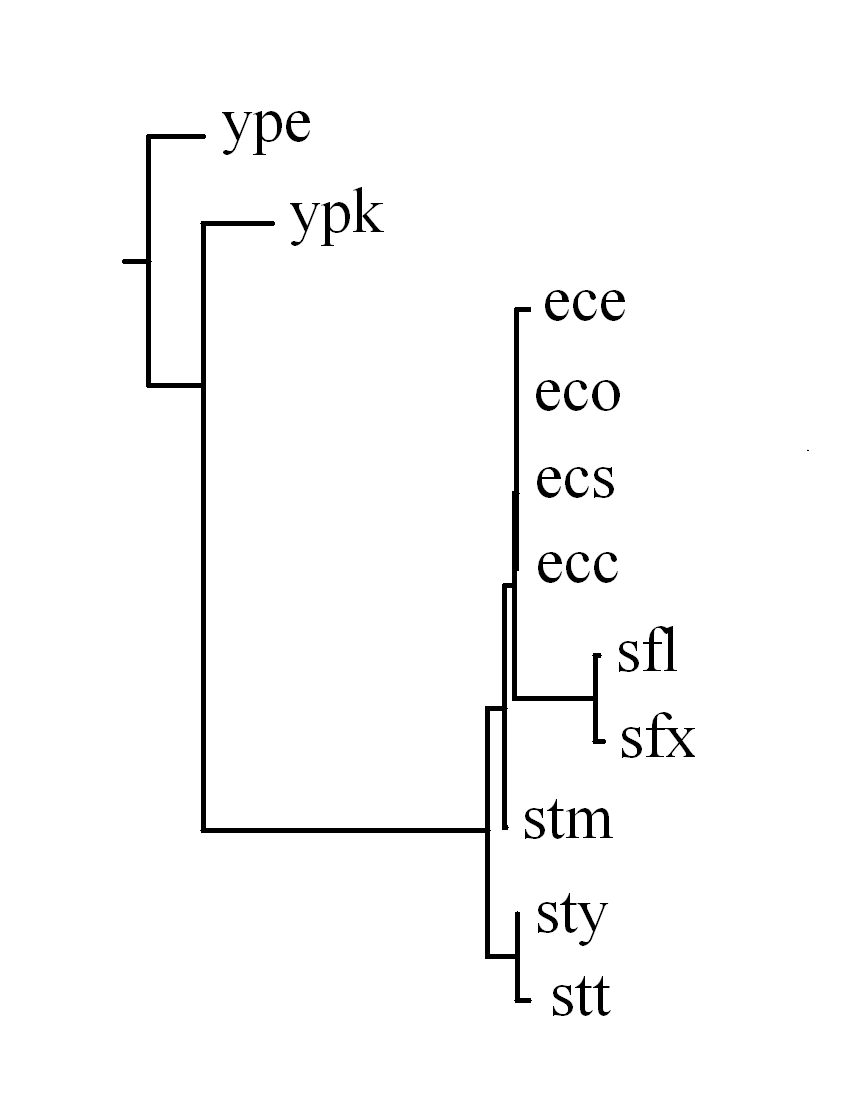
Moreover, the calculated
breakpoint/rearrangement distance between
V. vulnificus and V. parahaemolyticus is smaller
than that between V. vulnificus and V. cholerae and
that between V. parahaemolyticus and V. cholerae,
which agrees with the previous results obtained by
Chen et al. (2003)
using other comparative genomics approach, and
by Lin et al. (2005)
and Lu et al. (2005) using block-interchanges only.
Table 4:
The breakpoint and rearrangement distance matrixes
for the first chromosomes of three
Vibrio pathogens
(click this link for
the detailed SPRING result).
| Breakpoint distance |
Rearrangement distance |
|
VP1 |
VV1 |
VC1 |
| VP1 |
- |
27 |
90 |
| VV1 |
27 |
- |
90 |
| VC1 |
90 |
90 |
- |
|
|
|
VP1 |
VV1 |
VC1 |
| VP1 |
- |
17 |
67 |
| VV1 |
17 |
- |
66 |
| VC1 |
67 |
66 |
- |
|
|
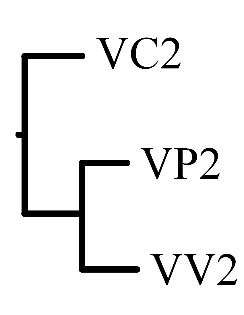
Table 5:
The breakpoint and rearrangement distance matrixes
for the second chromosomes of three
Vibrio pathogens
(click this link for
the detailed SPRING result).
| Breakpoint distance |
Rearrangement distance |
|
VP2 |
VV2 |
VC2 |
| VP2 |
- |
12 |
18 |
| VV2 |
12 |
- |
19 |
| VC2 |
18 |
19 |
- |
|
|
|
VP2 |
VV2 |
VC2 |
| VP2 |
- |
10 |
16 |
| VV2 |
10 |
- |
17 |
| VC2 |
16 |
17 |
- |
|
|
(3) Gene Orders of 29 gamma-Proteobacteria
In this experiment, we selected 29 gamma-proteobacteria
from the on-line supplementary material
provided by Belda et al.,
and ran SPRING using both reversals and block-interchanges
to infer their evolutionary trees according to their gene orders.
Please click this
link for its exprimental result in detail.
Consequently, the tree topology inferred by breakpoint distances
is very similar to that inferred by rearrangement distances, but
with two following differences.
Both the Shi. flexneri and Bl. floridanus strains
move closer to E. coli in the rearrangement-based topology.
The correlation coefficient between
the breakpoint and rearrangement distance matrixes is 0.997.
It is worth mentioning that in the rearrangement-based topology
inferred by Belda et al. (2005) using only reversals,
the Shi. oneidensis strains are away from the
three Pseudomonas species, which is contrary to
our rearrangement-based topology by considering both
reversals and block-interchanges.
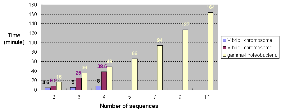
Currently, SPRING is installed on IBM PC with 2.8 GHz processor and
3 GB RAM under Linux system.
Figure 1 shows the time of running SPRING using
different number of chromosomal sequences of different
lengths ranging from 1.0~1.8 Mbp
(e.g., Vibrio chromosome II),
2.9~3.2 Mbp (e.g., Vibrio chromosome I)
and 4.5~5.5 Mbp (e.g., gamma-proteobacteria), respectively.
Figure 2 shows the time of running SPRING using different
number of the gene orders of 244 genes with/without showing
optimal scenarios.
Figure 1: The time of running SPRING using chromosomal sequences
|
Figure 2: The time of running SPRING using gene orders
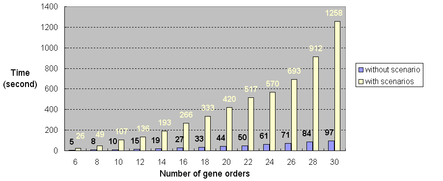
|
-
FASTA format:
A sequence in FASTA format starts with a single-line description, followed by lines of sequence data.
The description line starts with a right angle bracket (">") and is usually followed by the sequence
identifiers and description.
An example of a sequence in FASTA format is shown as follows.
>An example of a sequence in FASTA format
TGGAGTATTAACAGAAAATTGATACCAAACGAACAAAGTTAAGTATAAAAACCGCGTTTAAATAACCCAC
ATATTCTTCGATAAGGAGAAAACATTTTAAATATTACAGTGTCACTTATTTACAATGTAAAGCCACGTTT
-
FASTA-like format:
Similarly, a gene/landmark order in FASTA-like format starts with
a single-line description, followed by lines of signed integers,
which are separated by space(s), with each integer representing
a homologous gene or identical landmark on all input chromosomes.
The description line starts with a right angle bracket (">") and is
usually followed by the chromosome identifiers and description.
The following is an example of a gene/landmark order in FASTA format.
>An example of a landmark order in FASTA-like format
1 -19 2 20 -15 3 -17 -16 -9 -18 -13 7 5 -12 6 -8 10 -4 11 -14
Some examples of sequence data or gene-/landmark-order data for testing
SPRING are collected as follows.
-
Gene-/Landmark-Order Data
- Belda,E., Moya,A., Silva,F.J. (2005) Genome Rearrangement Distances and Gene Order Phylogeny in Gamma-Proteobacteria, Mol. Biol. Evol., 22, 1456-1467.
[PubMed]
- Chen,C.Y., Wu,K.M., Chang,Y.C., Chang,C.H., et al. (2003)
Comparative Genome Analysis of Vibrio Vulnificus, a Marine Pathogen, Genome Res., 13, 2577-2587.
[PubMed]
- Darling,A.C.E., Mau,B., Blattner,F.R. and Perna,N.T. (2004) Mauve: Multiple Alignment of Conserved Genomic Sequence With Rearrangement, Genome Res., 14, 1394-1403.
[PubMed]
- Lin,Y.C., Lu,C.L., Chang,H.Y. and Tang,C.Y. (2005) An
Efficient Algorithm for Sorting by Block-Interchanges and Its
Application to the Evolution of Vibrio Species, J. Comp. Biol., 12, 102-112.
[PubMed]
- Lin,Y.C., Lu,C.L. and Tang,C.Y. (2006) Sorting Permutation by Reversals with Fewest Block-Interchanges, manuscript.
- Lu,C.L., Wang,T.C., Lin,Y.C. and Tang,C.Y. (2005) ROBIN: A Tool for Genome Rearrangement of Block-Interchanges, Bioinformatics, 12, 2780-2782.
[PubMed]
- Mantin,I. and Shamir,R. (1999) An algorithm for sorting signed permutations by reversals. http://www.math.tau.ac.il/~rshamir/GR/